Model evaluation error metrics#
To evaluate different quality control methods, their results can be methodologically compared to raw data. For this, we provide several evaluation metrics which are desgined for skewed timeseries data. In the following, we explain three example evaluation metrics.
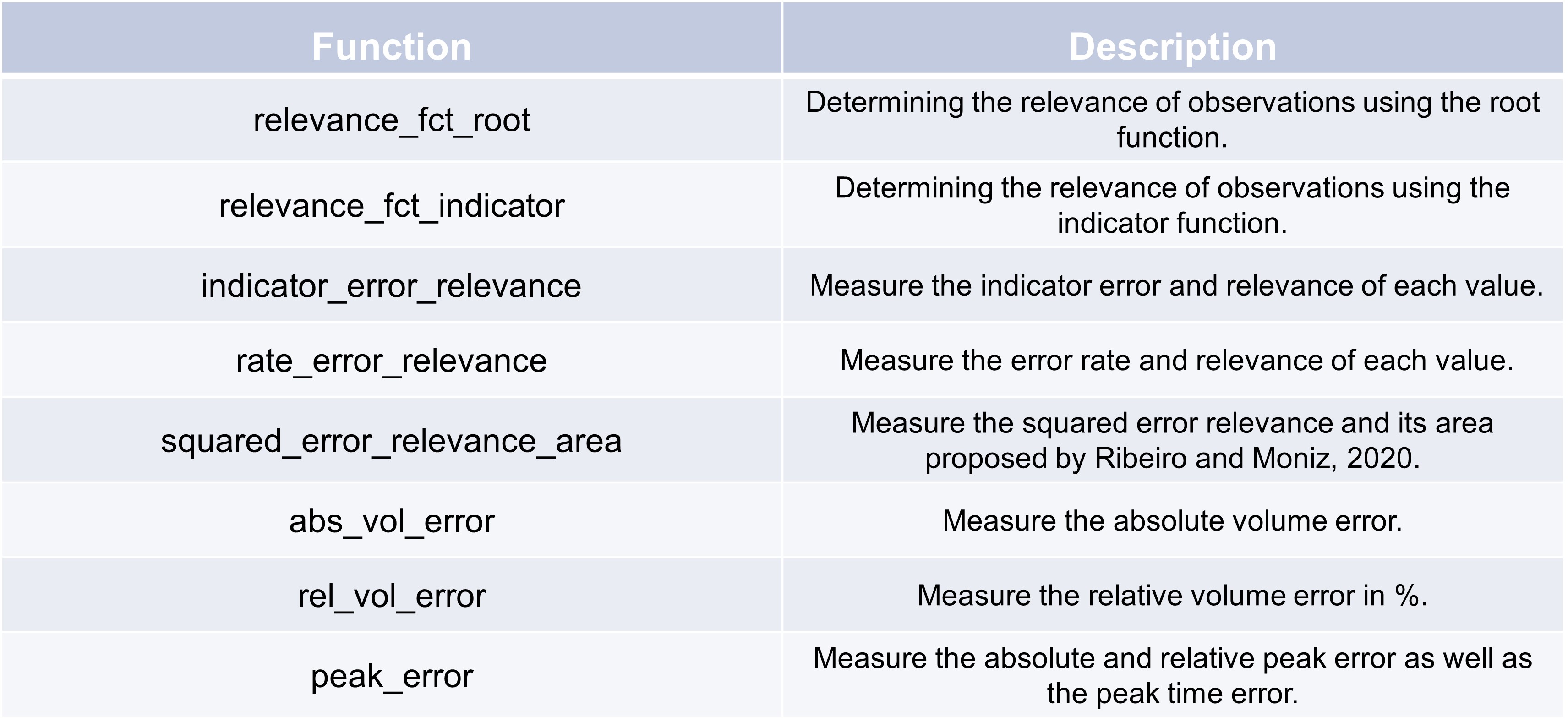
relevance_fct_root and relevance_fct_indicator can be used to determine the relevance of observations. They are
usually used within evaluation functions for a sample weighting.
indicator_error_relevance, rate_error_relevance, and squared_error_relevance_area can bu utilized
similar to, e.g. the MSE metric from scikit-learn for an evaluation of the whole dataset (maybe with sample weighting).
The last three evaluation metrics from the table, abs_vol_error, rel_vol_error, and peak_error
are usually applied on an event basis.
Dataset-based evaluation#
>>> y_gt = pd.Series([0, 1, 2, 1.25])
>>> y_pred = pd.Series([0, 0, 4, 1.26])
>>> print("Indicator error relevance + no weight. \t\t%.2f" % TSCC.assessment.indicator_error_relevance(y_gt, y_pred, (-float("inf"), 1), lambda y_gt: pd.Series([1] * len(y_gt))))
>>> print("Indicator error relevance + ind. weight. \t%.2f" % TSCC.assessment.indicator_error_relevance(y_gt, y_pred, (-float("inf"), 1), TSCC.assessment.relevance_fct_indicator, (1.25,float("inf"))))
>>> print("Indicator error relevance + root weight.\t%.2f" % TSCC.assessment.indicator_error_relevance(y_gt, y_pred, (-float("inf"), 1), TSCC.assessment.relevance_fct_root))
>>> print("MSE + ind. weight.\t\t\t\t%.2f" % sklearn.metrics.mean_squared_error(y_gt, y_pred, sample_weight = TSCC.assessment.relevance_fct_indicator(y_gt, (1.25, float("inf")))))
>>> print("Rate error relevance + ind. weight.\t\t%.2f" % TSCC.assessment.rate_error_relevance(y_gt, y_pred, TSCC.assessment.relevance_fct_indicator, (1.25,float("inf"))))
>>> print("SERA + root weight.\t\t\t\t%.2f" % TSCC.assessment.squared_error_relevance_area(y_gt, y_pred, TSCC.assessment.relevance_fct_root(y_gt))[0])
Indicator error relevance + no weight.          0.75
Indicator error relevance + ind. weight.        0.50
Indicator error relevance + root weight.        0.85
MSE + ind. weight.                              2.00
Rate error relevance + ind. weight.             0.50
SERA + root weight.                             5.00
Our data set to be evaluated consists of a ground truth series and a prediction series.
The first evaluation metric is the indicator_error_relevance metric without a weighting ob observations (equal weights).
The result is 0.75, because 3/4 of the observations are within the given maximal deviation 1 of y_gt
and y_pred. The second example also uses indicator_error_relevance metric but with a weighting by
relevance_fct_indicator. The binary weighting leads to a disregarding of observation 0 and 1. Observation 3 is
not withing the given maximal deviation, observation 4 is. The result is therefore 0.5. indicator_error_relevance
with the relevance_fct_root works in the same way besides its different observation weighting.
We also used the regular scikit-learn mean_squared_error with our custom relevance function.
Event-based evaluation#
First, a data set containing several events is created. Then, events are isolated using the TSCC.exploration.getEvents function. At last, different event-based evaluation metrics such as the absolute volume error are computed.
import pandas as pd
import numpy as np
from datetime import datetime, timedelta

# Generate sample data for demonstration
np.random.seed(0)

# Generate timestamps
start_time = datetime(2024, 1, 1)
end_time = datetime(2024, 1, 2)
num_samples = 25
timestamps = pd.date_range(start=start_time, end=end_time, periods=num_samples)

# Generate df_value_raw and df_value_gt using gamma distribution
shape_raw, scale_raw = 2., 10.  # Gamma distribution parameters for df_value_raw
shape_gt, scale_gt = 2.5, 10.5  # Gamma distribution parameters for df_value_gt
# Parameters for generating dependent values
mean_shift_raw = 0.2  # Mean shift for df_value_raw
mean_shift_gt = 0.3   # Mean shift for df_value_gt
autoreg_factor_raw = 0.7  # Auto-regressive factor for df_value_raw
autoreg_factor_gt = 0.8   # Auto-regressive factor for df_value_gt
# Generate df_value_raw and df_value_gt with auto-regressive behavior
df_value_raw = np.zeros(num_samples)
df_value_gt = np.zeros(num_samples)

for i in range(1, num_samples):
    df_value_gt[i] = mean_shift_gt + autoreg_factor_gt * df_value_gt[i - 1] + np.random.gamma(shape_raw, scale_raw)

df_value_raw = df_value_gt + np.random.normal(0, 5, num_samples)

# Create the DataFrame
df = pd.DataFrame({
    'timestamp': timestamps,
    'df_value_gt': df_value_gt,
    'df_value_raw': df_value_raw,
})

# Display the first few rows of the DataFrame
print(df.head())
            timestamp  df_value_gt  df_value_raw
0 2024-01-01 00:00:00     0.000000     -2.548261
1 2024-01-01 01:00:00    51.688296     49.497924
2 2024-01-01 02:00:00    64.035446     57.771469
3 2024-01-01 03:00:00   105.799679    109.687131
4 2024-01-01 04:00:00    91.905608     83.836119
event_list = TSCC.exploration.getEvents(df.set_index('timestamp')["df_value_gt"],
    max_time_dist_from_center = "120t",
    center_valley = (70, float("inf")),
    center_peak = (100, float("inf")),
    event_sum=(500, float("inf")),
         event_dist = (0.000001, float("inf"), .3))

for cur_event in event_list:
    print("Event characteristics (of ground truth)")
    print("Event start:\t\t", cur_event[0])
    print("Event end:\t\t", cur_event[1])
    print("Event min. intensity:\t%.2f" %  cur_event[2])
    print("Event max. intensity:\t%.2f" %  cur_event[3])
    print("Event sum:\t\t%.2f" %  cur_event[4])
    print()
    print("Evaluation results")
    df_event = df.query(f'"{cur_event[0]}" <= timestamp <= "{cur_event[1]}"')
    ave = TSCC.assessment.abs_vol_error(df_event.set_index("timestamp")["df_value_gt"], df_event.set_index("timestamp")["df_value_raw"])
    print("Absolute volume error:\t%.2f" % ave)
    rve = TSCC.assessment.rel_vol_error(df_event.set_index("timestamp")["df_value_gt"], df_event.set_index("timestamp")["df_value_raw"])
    print("Relative volume error:\t%.2f" % rve)
    ape, rpe, pte = TSCC.assessment.peak_error(df_event.set_index("timestamp")["df_value_gt"], df_event.set_index("timestamp")["df_value_raw"])
    print("Absolute peak error:\t%.2f" % ape)
    print("Relative peak error:\t%.2f" % rpe)
    print("Peak time error:\t", pte)
    print()
Event characteristics (of ground truth)
Event start:                    2024-01-01 06:00:00
Event end:                  2024-01-01 10:00:00
Event min. intensity:       94.20
Event max. intensity:       105.61
Event sum:                  510.93

Evaluation results
Absolute volume error:      -11.14
Relative volume error:      -2.18
Absolute peak error:         0.53
Relative peak error:         0.51
Peak time error:        -1 days +21:00:00
The output includes an event from 2024-01-01 06:00:00 to 2024-01-01 10:00:00 (based on the criteria set in TSCC.exploration.getEvents).
The absolute volume error of this event is -11.14 units (abs_vol_error), the prediction is 11.14 units less
than the ground truth. The relative error is -2.18`% (``rel_vol_error`).
The APE, RPE and PTE can be retrieved using peak_error.
The absolute peak error of the prediction in contrast to the ground truth is 0.53, the prediction is
therefore 0.53 units greater than the ground truth. The relative peak error is `0.51`%.
And the peak time is 3 hours earlier for the prediction than for the ground truth.